August 30th, 2017

从图像识别说起

起因在于之前邮件通信还占主流的时候，需要花费大量的时间和人力来清理和分发各种地方的信件，主要是通过上方的邮件编码，于是有人想到是否能通过计算机自动识别这些邮件编码来提高效率。经过不懈的努力，Yann LeCun 弄出了第一个手写数字的辨识程序，其中比较关键的就是卷积神经网络(Convolutional Neural Network, CNN)的架构。这个东西在当时有多大作用我不是很清楚，但是在现在的计算机视觉领域，CNN的影响力是非常大的。

局限于当时计算机的运算能力，这个架构没有办法做得更加复杂，运用在其他的物体识别上表现不是很好，相关的研究也没有较大的突破。直到2012年的 ImageNet挑战赛分类问题上，CNN架构的一个模型(AlexNet)获得了这个挑战的冠军，并且把错误率从25.8%下降到了16.4%，这时候人们才开始认识到CNN的优势。之后的几年中，CNN的架构越来越多，也使用了很多方法和技巧让网络越来越深的同时提高准确率。

下面先用一个例子看CNN的架构，这个代码中使用了VGG19模型，这个架构是2014年ImageNet挑战赛分类问题的亚军

20170830_1

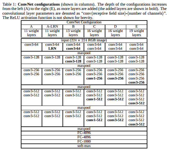
使用VGG19进行图像分类

这里主要参考了大佬的代码，应该还比较好懂吧

代码链接: https://github.com/BIGBALLON/cifar-10-cnn/blob/master/3_Vgg19_Network/Vgg19_keras.py

讲解：https://zhuanlan.zhihu.com/p/28346839

由于数据集使用的是cifar10，所以需要对架构进行一些修改，主要是最后的全连接层的节点数量有变化。

主要的模型建立代码如下（使用keras，后端使用的是tensorflow）：

前端后端只是一种形象的说法。由于tensorflow的代码实现起来有点复杂，而Keras提供简洁一致的API，能帮助用户快速实现神经网络。可以简单的看成keras是tensorflow（以及Theano等）的封装

def conv_layer(filters, kernel_size, name, input_shape=None):
    params = {
        "filters": filters,
        "kernel_size": kernel_size,
        "padding": 'same',
        'kernel_regularizer': keras.regularizers.l2(weight_decay),
        'kernel_initializer': he_normal(),
        'name': name
    }
    if input_shape is not None:
        params['input_shape'] = input_shape
    return Conv2D(**params)

def build_model():
    model = Sequential()

    # Block 1
    model.add(conv_layer(64, 3, 'block1_conv1', x_train.shape[1:]))
    model.add(BatchNormalization())
    model.add(Activation('relu'))

    model.add(conv_layer(64, 3, 'block1_conv2'))
    model.add(BatchNormalization())
    model.add(Activation('relu'))

    model.add(MaxPooling2D((2, 2), strides=(2, 2), name='block1_pool'))

    # Block 2
    model.add(conv_layer(128, 3, 'block2_conv1'))
    model.add(BatchNormalization())
    model.add(Activation('relu'))

    model.add(conv_layer(128, 3, 'block2_conv2'))
    model.add(BatchNormalization())
    model.add(Activation('relu'))

    model.add(MaxPooling2D((2, 2), strides=(2, 2), name='block2_pool'))

    # Block 3
    model.add(conv_layer(256, 3, 'block3_conv1'))
    model.add(BatchNormalization())
    model.add(Activation('relu'))

    model.add(conv_layer(256, 3, 'block3_conv2'))
    model.add(BatchNormalization())
    model.add(Activation('relu'))

    model.add(conv_layer(256, 3, 'block3_conv3'))
    model.add(BatchNormalization())
    model.add(Activation('relu'))

    model.add(conv_layer(256, 3, 'block3_conv4'))
    model.add(BatchNormalization())
    model.add(Activation('relu'))

    model.add(MaxPooling2D((2, 2), strides=(2, 2), name='block3_pool'))

    # Block 4
    model.add(conv_layer(512, 3, 'block4_conv1'))
    model.add(BatchNormalization())
    model.add(Activation('relu'))

    model.add(conv_layer(512, 3, 'block4_conv2'))
    model.add(BatchNormalization())
    model.add(Activation('relu'))

    model.add(conv_layer(512, 3, 'block4_conv3'))
    model.add(BatchNormalization())
    model.add(Activation('relu'))

    model.add(conv_layer(512, 3, 'block4_conv4'))
    model.add(BatchNormalization())
    model.add(Activation('relu'))

    model.add(MaxPooling2D((2, 2), strides=(2, 2), name='block4_pool'))


    # Block 5
    model.add(conv_layer(512, 3, 'block5_conv1'))
    model.add(BatchNormalization())
    model.add(Activation('relu'))

    model.add(conv_layer(512, 3, 'block5_conv2'))
    model.add(BatchNormalization())
    model.add(Activation('relu'))

    model.add(conv_layer(512, 3, 'block5_conv3'))
    model.add(BatchNormalization())
    model.add(Activation('relu'))

    model.add(conv_layer(512, 3, 'block5_conv4'))
    model.add(BatchNormalization())
    model.add(Activation('relu'))

    # model modification for cifar-10
    model.add(Flatten(name='flatten'))
    model.add(Dense(4096, use_bias = True, kernel_regularizer=keras.regularizers.l2(weight_decay), kernel_initializer=he_normal(), name='fc_cifa10'))
    model.add(BatchNormalization())
    model.add(Activation('relu'))
    model.add(Dropout(dropout))
    model.add(Dense(4096, kernel_regularizer=keras.regularizers.l2(weight_decay), kernel_initializer=he_normal(), name='fc2'))  
    model.add(BatchNormalization())
    model.add(Activation('relu'))
    model.add(Dropout(dropout))      
    model.add(Dense(10, kernel_regularizer=keras.regularizers.l2(weight_decay), kernel_initializer=he_normal(), name='predictions_cifa10'))        
    model.add(BatchNormalization())
    model.add(Activation('softmax'))

    # load pretrained weight from VGG19 by name      
    model.load_weights(filepath, by_name=True)

    sgd = optimizers.SGD(lr=.1, momentum=0.9, nesterov=True)
    model.compile(loss='categorical_crossentropy', optimizer=sgd, metrics=['accuracy'])
    return model

基本上就是不停的堆积卷积层，用BatchNormalization然后使用relu激活函数。堆积的方法和技巧我还没太弄明白，这里是直接用的别人的架构所以不涉及到模型的设计，如果是自己设计架构的话就需要考虑怎么拼好这个积木了。

剩下的代码主要就是使用Keras的一些技巧了，具体可以参照Keras文档。这里的主要步骤是加载数据集并预处理，配置TensorBoard，动态调整learning rate，对图像进行随机水平旋转和图像偏移。

完整代码地址：https://github.com/junmo1215/practice/tree/master/vgg19_for_cifar10

最终的准确率在93%左右，如果进一步使用调整weight_decay可以达到94.14%，具体参考这篇文章：https://zhuanlan.zhihu.com/p/28346839

我和这篇文章的做法还有一点区别是数据预处理的时候没有除以标准差，主要也是想看看有没有什么区别

在图像处理中，由于像素的数值范围几乎是一致的（都在0-255之间），所以进行这个额外的预处理步骤并不是很必要。

https://zhuanlan.zhihu.com/p/21560667?refer=intelligentunit

http://cs231n.github.io/neural-networks-2/

中间层可视化

虽然vgg19的架构取得了很好的效果，但是比较困扰我的是这个架构是怎么设计出来的，在中间的每一层都发生了什么，后来搜了一下，这个叫做Deep Visualization，相关的paper是 Visualizing and Understanding Convolutional Networks 和 Understanding Neural Networks Through Deep Visualization

对于中间层可视化这部分我目前还没有研究的很透，当时只是用了一个工具看了下每一层的画面是什么样的，大概能保留多少的内容。工具地址：https://github.com/jakebian/quiver(模型需要是用Keras搭好的)。不过这个最后出来的结果跟我想要的有些不一样，之后可能会深入的看一下这个方面。

另一个有点相关的技术是Deep Dream，也还没有仔细看

风格迁移

风格迁移我看到最早的一篇paper是 A Neural Algorithm of Artistic Style，介绍了风格迁移的主要思路。

风格迁移大致来讲是生成一张图，在内容上跟 content_image 相近，在风格上跟 style_image 相近。这篇paper的作者尝试使用原有的分类模型来提取图像的内容和风格，并取得了不错的效果。大概思路就是原有分类模型（比如VGG19等）的某一层能比较代表图像的内容，某几层会比较代表风格，所以采用缩小生成图像和原始图像的这几层差异的方式让生成的图像越来越符合要求。所以loss function就是 result_image 与 content_image 在内容层feature的差异 + result_image 与 style_image 在风格层feature的差异。只需要经过迭代让这个loss减小就能逐渐取得一个比较好的效果。

content_loss的定义是两个图片在这一层的feature逐个比较差异，然后取平方相加，style_loss略微有些不同，是对相应层的feature求一个Gram矩阵，再对这个矩阵中的每一个元素逐个比较取平方相加。

计算content_loss和style_loss的代码如下：

def content_loss(content_features, result_features):
    """
    Compute the content loss for style transfer.
    
    Inputs:
    - result_features: features of the current image, Tensor with shape [1, height, width, channels]
    - content_features: features of the content image, Tensor with shape [1, height, width, channels]
    
    Returns:
    - content loss
    """
    return tf.reduce_sum((content_features - result_features)**2)

def gram_matrix(features):
    """
    Compute the Gram matrix from features.
    
    Inputs:
    - features: Tensor of shape (1, H, W, C) giving features for
      a single image.

    Returns:
    - gram: Tensor of shape (C, C) giving the
      Gram matrices for the input image.
    """
    shape = tf.shape(features)
    H, W, C = shape[1], shape[2], shape[3]
    F = tf.reshape(features, (H*W, C))
    G = tf.matmul(F, F, transpose_a=True)
    # normalize 
    G /= tf.cast(H * W * C, tf.float32)
    return G

def style_loss(result_features, style_features):
    """
    Computes the style loss at a set of layers.
    
    Inputs:
    - result_features: features of the current image, Tensor with shape [1, height, width, channels]
    - style_features: features of the style image, Tensor with shape [1, height, width, channels]

    Returns:
    - style_loss
    """
    A = gram_matrix(result_features)
    G = gram_matrix(style_features)
    return tf.square(tf.norm(A - G))

虽然论文没有提到，但是在实作中，为了让图片更加平滑，减少噪点，会增加一个tv_loss，是计算相邻像素之间的差异

def tv_loss(img):
    """
    Compute total variation loss.
    
    Inputs:
    - img: Tensor of shape (1, H, W, 3) holding an input image.
    
    Returns:
    - loss
    """
    # 这部分是为了减少每个图片相邻像素的差异，让图片更加平滑，减少噪点
    shape = tf.shape(img)
    H = shape[1]
    W = shape[2]
    diff0 = tf.slice(img, [0, 0, 1, 0], [1, H-1, W-1, 3]) - tf.slice(img, [0, 0, 0, 0], [1, H-1, W-1, 3])
    diff1 = tf.slice(img, [0, 1, 0, 0], [1, H-1, W-1, 3]) - tf.slice(img, [0, 0, 0, 0], [1, H-1, W-1, 3])
    loss = tf.square(tf.norm(diff0)) + tf.square(tf.norm(diff1))
    return loss

核心地方就是定义了这个loss function，接下来就是迭代使这个loss最小。完整代码地址： https://github.com/junmo1215/practice/tree/master/style_transfer

代码参照CS231n(Spring 2017) assignment3 StyleTransfer-TensorFlow.ipynb

风格迁移在这篇paper之后又有很多新的发展，这里实作的只是最基础的一个版本。更多的内容可以参考这个地址: https://github.com/ycjing/Neural-Style-Transfer-Papers

个人觉得有用的一些小技巧：

初始化的时候不用随机噪点，使用content_image初始化效果会好些

可以尝试把content_image或者style_image变成空白图像感受下这个网络的输出

迭代一定步骤之后输出图像，对比图像之间的差异决定迭代的次数

参考

machine-learning (21)

junmo

首页

分类

标签

链接

[实作]从图像分类到风格迁移

从图像识别说起

使用VGG19进行图像分类

中间层可视化

风格迁移

参考

首 页

分 类

标 签

链 接

[实作]从图像分类到风格迁移

从图像识别说起

使用VGG19进行图像分类

中间层可视化

风格迁移

参考

首页

分类

标签

链接